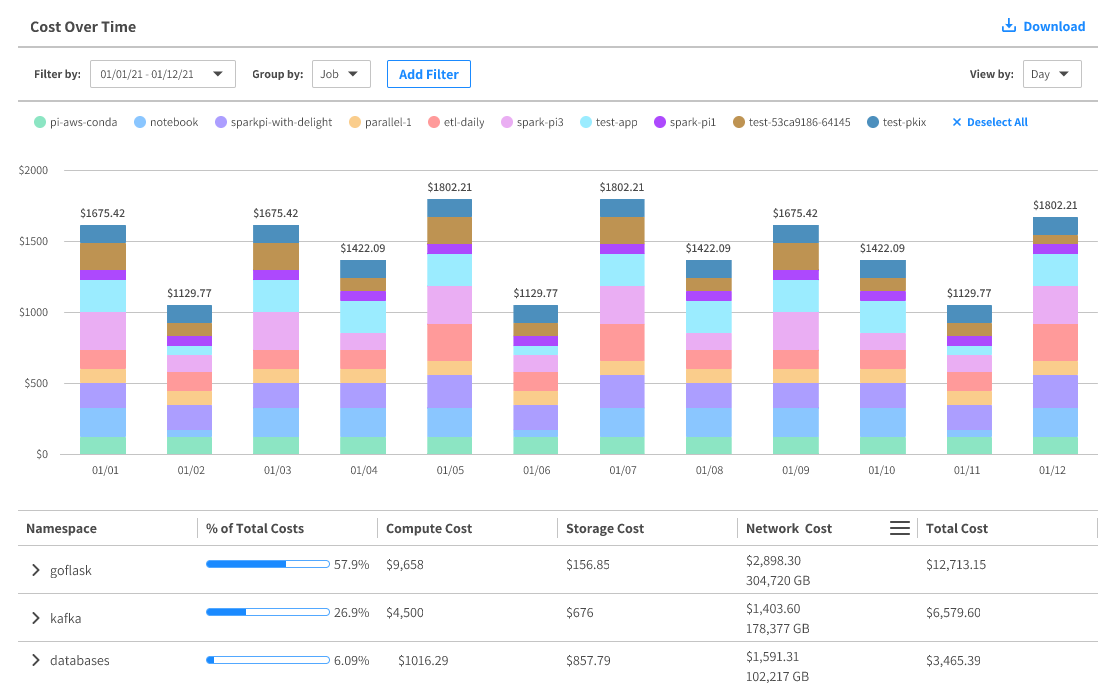
Cost Analysis
In a containerized Kubernetes environment, where multiple services and applications run on shared infrastructure, isolating the cost of each component, whether an app, service, or environment, can be challenging.
Ocean breaks down cluster infrastructure costs, provides insights across layers, and helps analyze application spend and perform chargebacks, without needing extensive resource tagging
Instead of viewing the total cost of a cluster, you can view costs broken down by namespaces and individual workloads, filter by container labels and annotations, and view compute and storage costs for each workload. This helps you understand your cloud infrastructure spend and manage expenses more effectively.
- For ECS only, costs are broken down by services, not namespaces.
- Only AWS Kubernetes cost analysis includes network costs.
How it Works
Ocean calculates compute and storage costs by breaking them down into their sources. It considers all workloads in the cluster and distributes managed infrastructure costs proportionally, based on each workload’s relative weight.
Compute Costs
To calculate cluster costs, Ocean follows this process:
- Ocean aggregates CPU and memory requests for each workload every hour, using data from the container orchestrator.
- It calculates the total managed infrastructure cost across spot, reserved, and on-demand instances.
- Based on these costs and workload resource requests, Ocean assigns costs to each workload proportionally.
For example, if a workload requests 20% of the cluster’s allocatable resources and the total cost is $100, that workload’s cost is $20
Ocean assigns cost weights based on two key factors:
- The cloud provider’s pricing difference between vCPU and memory.
- The CPU-to-memory ratio in the cluster, which indicates whether the cluster is more CPU-optimized or memory-optimized. vCPU and memory are the main elements of cluster resource allocation.
Depending on the instance type and family, 1 vCPU can cost between 7 to 13 times more than 1 GiB of memory.
In addition, a cluster that is optimized for memory, using more memory optimized instances, should have a higher weight for memory compared to a cluster optimized for CPU, using more CPU optimized instances.
For example, in two clusters, Cluster-1 (memory optimized) and Cluster-2 (CPU optimized):
- Cluster-1 with 40 vCPU and 320 GiB memory (1:8 CPU:memory ratio)
- Cost weight for Compute (vCPU) = 48% and memory (GiB) = 52%
- Cluster-2 with 120 vCPU and 120 GiB memory (1:1 CPU:Mem ratio)
- Cost weight for Compute (vCPU) = 91% and memory (GiB) = 9%
In Cluster-1, if workload-1 requests resources for 2 vCPUs and 12 GiB of memory, and the total cluster allocatable resources are 40 vCPUs and 320 GiB of memory, then the resource allocation of that workload is:
Resource allocation = (0.48 * 2/40) + (0.52 * 12/320) = 0.044 or 4.4%
Workload-1 used 4.4% of the total cluster allocatable resources. Workload-1 will be assigned 4.4% of Cluster-1 compute costs.
In Cluster-2, if workload-2 requests resources for 4 vCPUs and 6 GiB of memory, and the total cluster allocatable resources are 120 vCPUs and 120 GiB of memory, then the resource allocation of that workload is:
Resource allocation = (0.91 * 4/120) + (0.09 * 6/120) = 0.035 or 3.5%
Workload-2 used 3.5% of the total cluster allocatable resources. Workload-2 will be assigned 3.5% of Cluster-2 compute costs.
Headroom and Idle Resources
Headroom is included in Ocean’s cost analysis and appears as a separate line item. It is distinct from idle resources because headroom represents intentionally reserved capacity to support scaling and workload stability, while idle resources refer to unused allocations that were not consumed by active workloads. Separating the two helps clarify which costs are strategic versus potentially wasteful.
Storage Costs
Ocean reflects Persistent Volume (PV) storage costs from AWS EBS or GCP Persistent Disks, using the following process:
- Ocean collects hourly usage data, including volume size, volume ID, and price per hour.
- Ocean calculates Persistent Volume Claim (PVC) costs: a. For each pod with PVCs, Ocean calculates cost as (pod run time) × (storage pricing), using the corresponding PV object, and its mapped volume. b. It then sums the PVC costs for each pod.
- Ocean displays storage costs broken down per workload, per hour. For standalone pods, it aggregates, and shows their total storage costs separately.
Root Volume Costs
To provide a comprehensive view, AWS EBS volumes attached to cluster node instances, but not used as Persistent Volumes (PVs), are also included in the storage cost analysis. These costs are divided evenly among all workloads running on the instance, ensuring fair distribution, and full visibility into infrastructure spend.
EFS Costs (for AWS only)
Ocean also includes Elastic File System (EFS) storage costs. These are calculated based on Amazon’s storage classes, and throughput pricing, as described on the Amazon EFS Pricing page.
To connect EFS storage costs to workload breakdowns, Ocean performs the following:
- Fetches hourly cost of EFS entities in the AWS account.
- Maps pods to their EFS of usage on an hourly basis, using the following logic: a. Ocean identifies pods using EFS storage by identifying certain properties defined on the PVC they are connected to. For a Kubernetes deployment, the PVC is the same for all replicas, and therefore, the storage cost per pod is split between the number of replicas run that hour. b. For the relevant pods identified, Ocean evenly spreads the cost between the different workloads that were using the EFS. In cases where a single EFS serves multiple applications (workloads) in the cluster or across different clusters, Ocean also spreads the cost evenly between the different workloads.
To retrieve the necessary EFS information, Ocean requires the following permission in the Access Policy:
elasticfilesystem:DescribeFileSystems
Network Costs (for AWS Kubernetes only)
Ocean network costs measure data transfer costs (in $) and bandwidth usage (in GB) for Kubernetes applications.
To enable network costs, install the network client (agent), which runs as a DaemonSet on every node in the Kubernetes cluster.
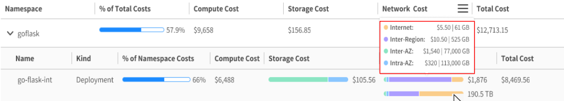
Ocean identifies and attributes cloud provider data transfer costs to Kubernetes applications, based on the following categories.
-
Internet: When an application sends traffic to an external IP address, outside the cloud provider, it incurs Internet data transfer costs, based on the amount of data (in GB) sent. For example, a streaming service delivering videos to external users, or a sales app backing up data to a private cloud. Cloud providers do not charge for incoming internet traffic.
-
Inter-Region: When traffic crosses regional boundaries, such as between North America and Europe, it incurs Inter-Region data transfer costs, based on the volume of data sent. The cost typically depends on the source region of the application generating the traffic.
-
Inter-AZ: When traffic moves between availability zones (AZ) within the same region, both ingress and egress directions are charged. This means both the source, and destination workloads, incur Inter-AZ data transfer costs, based on the amount of data transferred.
-
Intra-AZ: Traffic within the same AZ is usually free. However, if an application accesses services using public IPs, such as DNS, Ingress, Load Balancer, Transit Gateway, or NAT Gateway, cloud providers may apply Inter-AZ-like charges. Examples include:
- DNS or Ingress resolving to a public IP.
- Load balancer traffic routed via NodePort public IP, instead of private pod IP, or ClusterIP.
If all application traffic stays within the cluster, in the same availability zone (AZ), and only private IPs are used, Ocean will show some Intra-AZ bandwidth usage, but the cost will be $0.00.
The network costs anaysis architecture is shown below.
The Ocean network client is installed in the Kubernetes cluster and runs as a Kubernetes DaemonSet on each node. It includes an exporter, and an eBPF packet counter, which collect network flow metrics from pods on the node. These metrics are sent, at regular intervals, to the Ocean backend cluster (AWS), for network cost calculation and aggregation, which can be retained for up to 90 days.
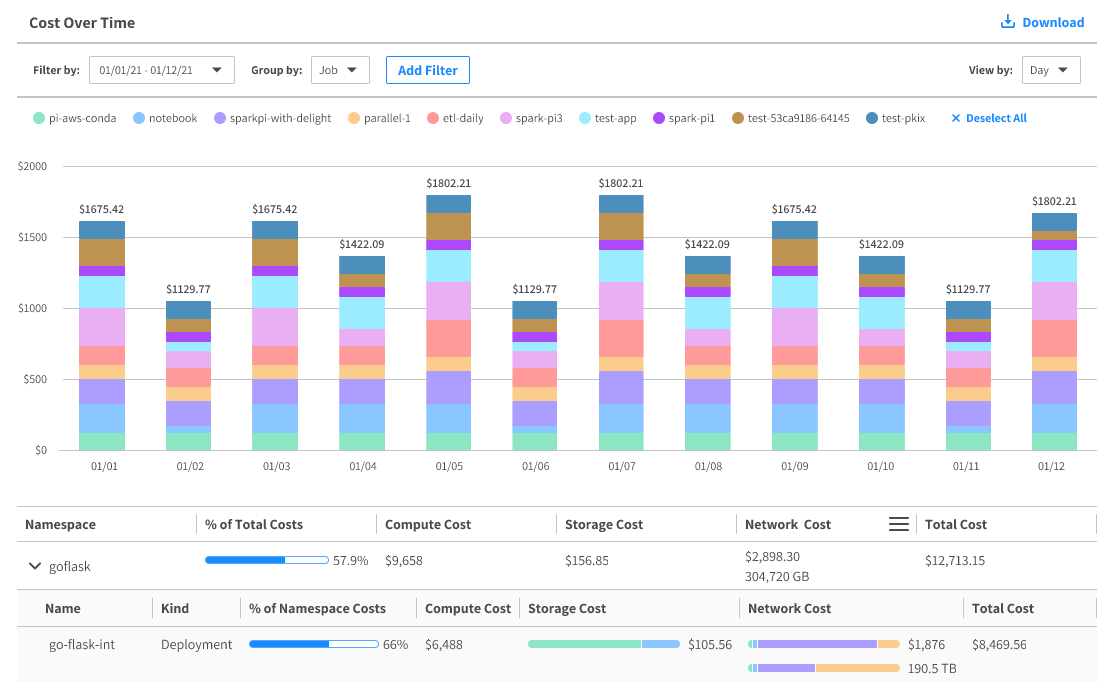
Breakdown Types
By default, Ocean shows cost breakdowns per workload, such as Kubernetes deployments. However, you can also view itemized costs by labels, and annotations. This is a powerful tool that lets you analyze cluster usage by department, application, function, such as development, testing, production, or any labeling system you’ve implemented.
The breakdown also includes cost information for different Kubernetes elements, or Kinds, such as Deployment, DaemonSet, StatefulSet, and Job
Captured Data Scope
Ocean captures and displays data only from instances (nodes) that are managed by Ocean. If your cluster includes instances that are not managed by Ocean, those instances are excluded from the analysis.